Chandoo.org Facing Downtime - 403 Error

GoDaddy which hosts my site (http://chandoo.org) just sent me an email saying chandoo.org is consuming way too much server resources and hence needs to be disabled. They didn't give me any time to move the site or disable plugins that might be causing excessive server load.

I have spoken with the customer care and they couldn't help me much since it is late in the night. I am hoping to get the site back up by tomorrow morning 9 AM PST.


For the time being I have pointed the RSS Feed source to r1c1.blogspot.com where I used to write about excel really long time back. I will post updates about chandoo.org here.

Stay tuned.

You can mail me at chandoo.d at gmail.com.

Howto: Excel Based Mutual Fund Portfolio Tracker

Instead of searching for the NAVs of all my funds at MyIRIS or MutualFundsIndia, I have developed a small excel sheet which will fetch the values for me and displays the current portfolio value at the click of a button. Here I am trying to share the "HOWTO" of the same.

1. Create an excel workbook with 2 sheets. Call one as "NAVs" and the other as "Portfolio".
2. In the NAVs sheet, click at one of the top-left cells (I did on A2), and go to Data -> Import External Data -> New Web Query. [For more information on using Web Queries, visit Using Web Queries to Import Data to Excel @ R1C1.
3. Now paste the url http://finance.indiamart.com/markets/mutual_funds/latest_mf_navs.html in Address box and press go. You would see something like this.
   
   Say "Import". Essentially what you have done is, creating an automatically updatable NAV list in the NAVs sheet.
4. Now select all Schemes in the imported table and define a named range as "fund_names" for it. [Creating Named Ranges in Excel]
5. Now, go to "Portfolio" sheet and create a table like this.
   
   [Click on it to Zoom]
   
6. Next select the Fundname column (I have 32 rows, you can have as many as you wish) and go to Data->Validation. Enter the settings like this.
   
   
7. Formulas:
   >>> For Purchase Value[f3]: "=e3*d3"
   >>> For Current Value[h3]: "=g3*d3"
   >>> For Current NAV[g3]: "=IF(C3="",0,VLOOKUP(C3,NAVs!$A$6:$D$1634,3,FALSE))"
   essentially, looking up for the selected fund name in the NAVs sheet and returning the exact NAV to this cell only if a fund name is selected.
   >>> Gain / Loss[i3]: "=IF(ISERROR((H3-F3)/F3),"",(H3-F3)/F3)"
   to avoid DIV 0 messages.
8. At the end of the table you can add a TOTAL row and repeat the necessary formulas to get the total portfolio performance.
9. Now the portfolio tracker is done. Enter the fund data by selecting the fund name from drop down and number of units purchased, purchase NAV. Rest will be shown by the tracker.
10. Remember: everytime you open the workbook, go to "NAVs" sheet and refresh the data. [Select anywhere in the table, right click and say Refresh Data]

Now this is a very basic portfolio tracker. I am thinking of adding some VBA / Macro so that everytime the table is refreshed, the new values are written in a separate sheet called "Historical NAV" so that we can track the fund performance over a period of time by selecting a date (instead of current date). Also, if we can import benchmark indices on runtime, you can get relative performance metrics. Plus, some more analysis of fund performances (instead of mere total return) would reveal the risk-returns of the portfolio. Lets see if I can build such a thing in my spare time.

[Just in case you do not have time for all this, then you can access the workbook that I have created here: Portfolio Manager MFs India ]

Document Management Using Excel

Consulting assingments typically come with myriad view points and tonnes of information. It becomes critical to sift through the entire information to get a clear overview of the problem at hand. Sadly, nobody has the casestudy written. Everyone has their own share of information /data/documents.

Recently we had a client sharing with us an elaborate list of documents as part of one consulting engagements. There were more than a hundred documents (excels, ppts, docs and loads of zipfiles as well) and we had to go through the same along with meetings and conf. calls. During this I have realized that excel can help greatly in processing these documents in an organized way and help in gathering views from multiple parties.

So this post explains how it can be done. [Download the excel Document Management Using Excel]

1. First I got a list of all the document names in the target directory in a textfile. To get it; go to CMD window (start->run->cmd) and then go to the target directory (cd \[target directory path]) and then finally type (DIR /B/S > filenames.txt). You will have all the file names piped in to that folder.
2. Then I copied the contents of that text file to an excel sheet.
   
3. Then I created an user defined formula for reversing the contents of a cell. (read How to reverse cell contents)
4. Then, I have added Doctype, Location, Comments? and Reversed columns to the sheet next to filenames column.
5. In "Reversed" column (Column G), I have typed the following formula,
   
   
6. Now I need to know the type of document each line is having. This can be dervied the from the extension of the file (or lack of it would mean a dirctory). Extension of the file is the substring after the last "." in the filename. How do we know where is the last dot? Well, we dont, but we do know where the first dot is in the reversed string [or anystring, just write, find(".","somestrng.stritir.fdkfjsdk") and it will return the first dot location]. So, the document type formula is,
   =IF(ISERROR(FIND(".",RIGHT(B2,8))), "Directory", RIGHT(B2,FIND(".",G2)-1))
   Remember, column G has the reversed Strings.
7. Next is the Location of the document, The formula for this would be,
   =IF(C2="Directory",B2,LEFT(B2,LEN(B2)-FIND("\",G2)))
   "Column-C" has the document type.
8. Once this is done you will have a structure like this,
   
   
9. Now share the excel sheet with others [Tools -> Share Workbook ...] and let everyone add their comments on each file. Managing the collective understanding of the documents is easy now.

Type: Document Managment, Data Analytics, Macro, String Functions
Applicability: In Consulting engagements, Better management of time, effort and knowledge.
Excel Knowledge Required: Medium
Ease of Implementation: Medium

Kicka$$ In-Cell Graphs: No 1

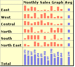
Eversince I discovered about Incell graphs in Juice Analytics sometime back, I was itching to use them and develop something fun, intuitive and easy. Work kept me buys for most of the last week, so I couldnt come up with something unique and simple till late yesterday. So here is something that I have come up with.

Using In-cell graphs to depict micro charts:

1. Learn how to create In-cell graphs at Juice Analytics. [Download Excel In-cell Graph Ideas from Juice Analytics]Its simple. If you have a monthly sales figure or someother number then you can convert it into incell graph using Rept() function. For example:
   Rept("#", 20) would result in ####################
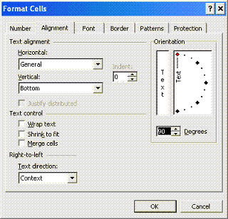
2. But Incell graphs are by default horizontal. Well, thats where you use text orientation feature of Excel. Goto Format->Cells->Alignment Tab. Change the orientation for the cells to 90 Degrees like shown here. You can display incell charts vertically now.
   
   
3. Essentially what you need to do to get something similar to the topmost figure is:
   --- Create Rept("|", monthly_sales_value OR something_else)
   --- Concatenate the results in to one cell along with Carriage return between each value (Quick tip on howto: "a" & char(10) & "b" will return the formula result in 2 lines; that is if you enable wrap text)
   --- Format the text to orient vertically
   
   
4. Playing with In-cell graphs: You can concatenate total values on the top of each graph, you can show average sales, max sales, min sales in seperate columns or together with "AVG", "MIN", "MAX" added in the end of the bar. If bars are too lengthy / small, you can divide or multiple with a constant. So on... [Download Excel In-cell Graph Ideas from Juice Analytics]

Remember: If you dont enable "Wrap Text" you wont get the desired effect.

Type: Tutorial, Graphs, Visualization, Data Representation
Applicability: To get that extra WOW effect, raise a few eye brows in conference rooms, Printed reports, Where data is more and graphs become useless
Excel Knowledge Required: Low to Medium
Ease of Implementation: Simple

Using Web Queries to Import Data to Excel

The other day, I bumped upon this powerful and really simple tool in excel. I must say, its one of those gems that is kept inside excel. I felt like a kid getting excited discovering a candy in his pant pockets. Well, to the point now!

Often, business data and analytics deal with lots of Ctrl+C, Ctrl+Vs. For example you might be downloading a financial statement from Google Finance or a rating for a select list of companies form Fitch! or AM Best or even simple top 250 movies list from IMDB. What we generally do is open the web page and copy/paste the data on to our excel sheets. In the end when we perform the analysis and conclude something, it is always "as of some past date". Well, with the help of Web Queries, the analytics can be real time, well, almost.

5 Steps to using Web Queries to Import Data to Excel Sheets:

1. First up, locate [Just locate, you need not load that page in excel] the site / webpage you want the data to be copied from. Remember, this should be on public domain without login access. Simply put, if you type the URL in the browser, the page should load, no matter whether you are logged in to that site or not. (Ex: IMDB Top 250 Movies)
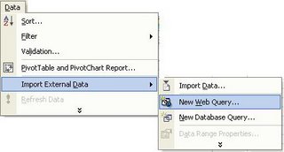
2. Open Excel. Go to Data -> Import External Data -> New Web Query
   
   
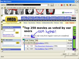
3. In the Dailog box for webquery enter the URL you want and say 'Go'.
   
   Select the table you want like this. The table outline would turn 'Green' or something differant. Click on it and you would see the mark becoming like a tick like this.
4. Say Import. In the next dailog enter the starting cell. You can click on the properties to change the behaviour of webimport, but it may not be necessary. While the import is going on you see a cyan colored globe trotting around itself on the status bar. If you cant, blame your office vendor.
5. Once the table is loaded, you can right click anywhere on it and say Refresh Data! and it would fetch the new data from web automatically.

Potential Applications of Web Queries Data Import Tool:

• Automated Portfolio Managers: Enable automatic refresh on File open and load MF, Share price related data from public sources.
• Realtime graphs, Charts and dash boards: You might have some application running on your LAN and generating data. Now assume there is a way to convert such data into HTML on the fly. Bingo! you dont have to copy paste the data to excel now. Just link up once and you are done.
• So many more, I think of almost anything and I see a possibility of using Web Query Imports to simplify that task.

Teaser for the weekend: How to get Graphs on Maps in Excel

[Click on the image for a bigger version]

Often business data goes hand in hand with geographical data. Thanks to tools like Google Maps and several associated mash-ups. But often it might be required to show data on a map to create an effect or draw some conclusions.

An example: Lets say you are analyzing annual sales in various States of US. Now usual ways of doing it include tables, bar/pie charts etc. But much more intuitive way would be to use an US outline map with bubbles in each state with their sizes representing segment/product-wise sales.

I had to do a similar analysis sometime back. And I did it in our dear excel itself without much pain (well, it is not so straightforward, but pretty much do-able)

So, here is a teaser for all the R1C1 readers. Try to findout the way for getting the following above graph in excel. No macros used (although, some amount of manual labour was!) The 3 colored bubbles represent 3 different segment/product figures (be it sales, profits, employees or anything you like).

Leave a comment with outline solution if you have one, Or wait till next week to find a simple enough way to do this.


Type: Teasers, Graphs, Data Analytics, Data Representation, Visualization
Applicability: for situations with both {sales, profits, people} and geographical data
Excel Knowledge Required: Moderate to Advanced
Ease of Implementation: Medium


PS: from this post onwards, I will be including the above format table with every post. To make the usage of R1C1 better.

3 Steps to Create cool dashboards in excel

Dashboards are very common business monitoring tools, but creating them in excel with all the bells and whistles is not so easy. So here is a quick 1-2-3 on how to do it.

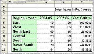
Lets take a sample of 2 consecutive year sales figures for 7 regions. The colums have Region name, 2004-05, 2005-06 figures and finally YoY Growth percentages. The lame dashboard should look something like this:


But may be we can make it little better. Ideally, a person looking at this would like (to know) the following things:

• What are the things that are going up / down / remaining constant
• The chart should look simple and not cluttered; meaning, there cant be multiple columns to present information. He/she should be able to look at one column and concluded something
• May be little graphics wont hurt the presentation while retaining the information.

So, a cool dashboard would look something like the below one:

Well, how to get it in 3 steps?

1. Type the following formula in the cell F5 and drag it to apply to all the cells
   
   [Click on the image to see bigger version of the formula]
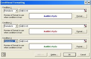
2. Select the range F5:F11, goto Format->Conditional Formatting and enter the following values there:
   
   [Click on the image to see bigger version of the formula]
   
3. Finally, if its already not, change the font of the worksheet to Arial, (see those arrow marks, they are not available in all fonts. And btw, if you dont know how to insert them in the formula use Start->Programs->Accessories->System Tools->Character Map and then locate the symbols.)

So, go ahead and impress everyone with the cool dashboards.